Fast Fourier Transform (FFT) Algorithm | Efficient Signal Processing

Description

The Fast Fourier Transform (FFT) is an efficient algorithm for computing the Discrete Fourier Transform (DFT) of a sequence. It converts a signal from the time domain to the frequency domain, revealing the frequency components that make up the signal. The FFT reduces the complexity of computing the DFT from O(n²) to O(n log n) by using a divide-and-conquer approach.

How It Works

Split the input signal into two parts:
- Elements at even positions
- Elements at odd positions
Apply FFT recursively to each half:
- Compute FFT of the even sequence
- Compute FFT of the odd sequence
Combine the results:
- Use roots of unity (twiddle factors) to combine transforms
- Apply combination formula for each frequency k
- First half: even[k] + t * odd[k]
- Second half: even[k] - t * odd[k]
The process continues recursively until:
- A sequence of length 1 is reached
- The FFT of a sequence of length 1 is itself

History

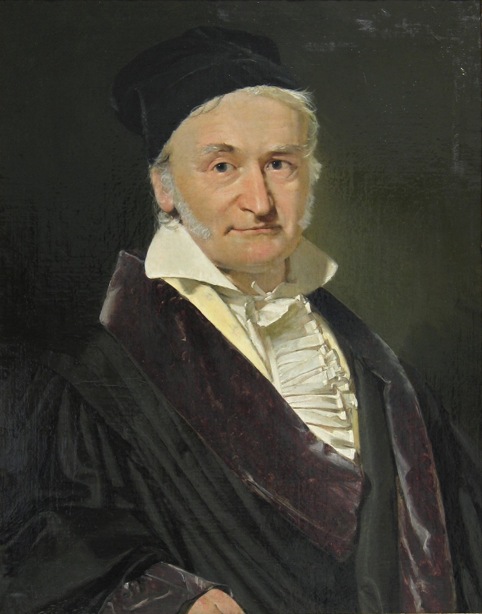
The Fast Fourier Transform has a rich history dating back to 1805 when Carl Friedrich Gauss first developed an algorithm for calculating the coefficients of a finite Fourier series. However, the modern FFT algorithm was popularized by James Cooley and John Tukey in their 1965 paper. Their algorithm, known as the Cooley-Tukey FFT algorithm, revolutionized digital signal processing by making Fourier analysis practical for computers. The algorithm was actually rediscovered, as Gauss's earlier work wasn't widely known. The development of the FFT is considered one of the most important algorithmic advances of the 20th century.

Visualization

Click Start to begin visualization

Implementation


import cmath

def fft(x):
    N = len(x)
    if N <= 1:
        return x
    
    # Divide
    even = fft(x[::2])
    odd = fft(x[1::2])
    
    # Combine
    T = [cmath.exp(-2j * cmath.pi * k / N) * odd[k] for k in range(N // 2)]
    return [even[k] + T[k] for k in range(N // 2)] + \
           [even[k] - T[k] for k in range(N // 2)]

# Example usage
if __name__ == "__main__":
    # Create a sample signal
    signal = [1, 2, 3, 4, 5, 6, 7, 8]
    result = fft(signal)
    
    print("Input signal:", signal)
    print("\nFFT result (magnitude):")
    for i, x in enumerate(result):
        print(f"Frequency {i}: {abs(x):.2f}")


#include <complex>
#include <vector>
using namespace std;

vector<complex<double>> fft(vector<complex<double>>& x) {
    int N = x.size();
    if (N <= 1) return x;
    
    // Divide
    vector<complex<double>> even, odd;
    for (int i = 0; i < N; i++) {
        if (i % 2 == 0) even.push_back(x[i]);
        else odd.push_back(x[i]);
    }
    
    even = fft(even);
    odd = fft(odd);
    
    // Combine
    vector<complex<double>> result(N);
    for (int k = 0; k < N/2; k++) {
        complex<double> t = polar(1.0, -2 * M_PI * k / N) * odd[k];
        result[k] = even[k] + t;
        result[k + N/2] = even[k] - t;
    }
    
    return result;
}

int main() {
    // Create a sample signal
    vector<complex<double>> signal = {1, 2, 3, 4, 5, 6, 7, 8};
    auto result = fft(signal);
    
    cout << "FFT result (magnitude):\n";
    for (int i = 0; i < result.size(); i++) {
        cout << "Frequency " << i << ": " 
             << abs(result[i]) << endl;
    }
    
    return 0;
}


using System.Numerics;

public class FFT {
    public Complex[] Transform(Complex[] x) {
        int N = x.Length;
        if (N <= 1) return x;
        
        // Divide
        var even = new Complex[N/2];
        var odd = new Complex[N/2];
        for (int i = 0; i < N/2; i++) {
            even[i] = x[2*i];
            odd[i] = x[2*i + 1];
        }
        
        even = Transform(even);
        odd = Transform(odd);
        
        // Combine
        var result = new Complex[N];
        for (int k = 0; k < N/2; k++) {
            double angle = -2 * Math.PI * k / N;
            Complex t = new Complex(Math.Cos(angle), Math.Sin(angle)) * odd[k];
            result[k] = even[k] + t;
            result[k + N/2] = even[k] - t;
        }
        
        return result;
    }
    
    public static void Main() {
        var fft = new FFT();
        
        // Create a sample signal
        var signal = new Complex[] {
            1, 2, 3, 4, 5, 6, 7, 8
        };
        
        var result = fft.Transform(signal);
        
        Console.WriteLine("FFT result (magnitude):");
        for (int i = 0; i < result.Length; i++) {
            Console.WriteLine($"Frequency {i}: {Complex.Abs(result[i]):F2}");
        }
    }
}

Complexity Analysis

Time Complexity

The time complexity is O(n log n), where n is the length of the input sequence:

Each level of recursion divides the problem size by 2
There are log n levels of recursion
At each level, we perform O(n) operations
Total: O(n) * O(log n) = O(n log n)

Space Complexity

The space complexity is O(n), which includes:

Recursion stack space: O(log n)
Storage for divided arrays: O(n)
Result array: O(n)

Advantages and Disadvantages

Advantages

Much faster than direct DFT computation
Widely used in signal processing applications
Enables efficient frequency analysis
Numerically stable implementation

Disadvantages

Input size must be a power of 2 for optimal performance
Complex implementation compared to DFT
Requires understanding of complex numbers
May have numerical precision issues

Quick Info

Fast Fourier Transform (FFT)